Finding and understanding relationships in data#
In today’s data-driven world, we are constantly bombarded with vast amounts of information. However, this raw data is often meaningless without the ability to identify relationships and patterns within it.
Finding and understanding relationships in data is crucial for making informed decisions, developing predictive models, and discovering new insights. Through the use of statistical techniques and machine learning algorithms, we can uncover hidden connections and dependencies between variables, enabling us to make accurate predictions and improve our understanding of complex systems.
Whether in business, science, or everyday life, the ability to analyze and interpret data is becoming increasingly important, and finding relationships within it is an essential skill for success.
How To#
import pandas as pd
df = pd.read_csv("data/housing.csv")
df.head()
| longitude | latitude | housing_median_age | total_rooms | total_bedrooms | population | households | median_income | median_house_value | ocean_proximity | |
|---|---|---|---|---|---|---|---|---|---|---|
| 0 | -122.23 | 37.88 | 41.0 | 880.0 | 129.0 | 322.0 | 126.0 | 8.3252 | 452600.0 | NEAR BAY |
| 1 | -122.22 | 37.86 | 21.0 | 7099.0 | 1106.0 | 2401.0 | 1138.0 | 8.3014 | 358500.0 | NEAR BAY |
| 2 | -122.24 | 37.85 | 52.0 | 1467.0 | 190.0 | 496.0 | 177.0 | 7.2574 | 352100.0 | NEAR BAY |
| 3 | -122.25 | 37.85 | 52.0 | 1274.0 | 235.0 | 558.0 | 219.0 | 5.6431 | 341300.0 | NEAR BAY |
| 4 | -122.25 | 37.85 | 52.0 | 1627.0 | 280.0 | 565.0 | 259.0 | 3.8462 | 342200.0 | NEAR BAY |
df.corr()
---------------------------------------------------------------------------
ValueError                                Traceback (most recent call last)
Cell In[2], line 1
----> 1 df.corr()

File /opt/hostedtoolcache/Python/3.8.18/x64/lib/python3.8/site-packages/pandas/core/frame.py:10054, in DataFrame.corr(self, method, min_periods, numeric_only)
  10052 cols = data.columns
  10053 idx = cols.copy()
> 10054 mat = data.to_numpy(dtype=float, na_value=np.nan, copy=False)
  10056 if method == "pearson":
  10057     correl = libalgos.nancorr(mat, minp=min_periods)

File /opt/hostedtoolcache/Python/3.8.18/x64/lib/python3.8/site-packages/pandas/core/frame.py:1838, in DataFrame.to_numpy(self, dtype, copy, na_value)
   1836 if dtype is not None:
   1837     dtype = np.dtype(dtype)
-> 1838 result = self._mgr.as_array(dtype=dtype, copy=copy, na_value=na_value)
   1839 if result.dtype is not dtype:
   1840     result = np.array(result, dtype=dtype, copy=False)

File /opt/hostedtoolcache/Python/3.8.18/x64/lib/python3.8/site-packages/pandas/core/internals/managers.py:1732, in BlockManager.as_array(self, dtype, copy, na_value)
   1730         arr.flags.writeable = False
   1731 else:
-> 1732     arr = self._interleave(dtype=dtype, na_value=na_value)
   1733     # The underlying data was copied within _interleave, so no need
   1734     # to further copy if copy=True or setting na_value
   1736 if na_value is not lib.no_default:

File /opt/hostedtoolcache/Python/3.8.18/x64/lib/python3.8/site-packages/pandas/core/internals/managers.py:1794, in BlockManager._interleave(self, dtype, na_value)
   1792     else:
   1793         arr = blk.get_values(dtype)
-> 1794     result[rl.indexer] = arr
   1795     itemmask[rl.indexer] = 1
   1797 if not itemmask.all():

ValueError: could not convert string to float: 'NEAR BAY'
df.total_rooms.corr(df.households)
0.9184844926543082
More than linear correlation#
from discover_feature_relationships import discover
rel = discover.discover(df.sample(500))
beyond_corr = rel.pivot(index="target", columns="feature", values="score").fillna(1)
beyond_corr
| feature | households | housing_median_age | latitude | longitude | median_house_value | median_income | ocean_proximity | population | total_bedrooms | total_rooms |
|---|---|---|---|---|---|---|---|---|---|---|
| target | ||||||||||
| households | 1.000000 | 0.037340 | -0.537450 | -0.518198 | -0.901268 | -0.949288 | -0.004915 | 0.657631 | 0.893712 | 0.760877 |
| housing_median_age | -0.314722 | 1.000000 | 0.050557 | 0.010672 | -0.340596 | -0.487119 | 0.066056 | -0.333395 | -0.454009 | -0.134160 |
| latitude | -0.336849 | -0.175834 | 1.000000 | 0.886597 | -0.386434 | -0.400958 | 0.371487 | -0.377302 | -0.496807 | -0.440968 |
| longitude | -0.379972 | -0.127651 | 0.857229 | 1.000000 | -0.477218 | -0.420772 | 0.296853 | -0.356622 | -0.531754 | -0.491624 |
| median_house_value | -0.489163 | -0.089184 | -0.201703 | 0.109102 | 1.000000 | 0.211742 | 0.227511 | -0.497541 | -0.571927 | -0.362765 |
| median_income | -0.471860 | -0.103471 | -0.293770 | -0.129196 | 0.320258 | 1.000000 | 0.026960 | -0.475921 | -0.481412 | -0.217507 |
| ocean_proximity | -0.521369 | -0.212248 | 0.210688 | 0.168251 | -0.309688 | -0.440625 | 1.000000 | -0.511484 | -0.525493 | -0.474652 |
| population | 0.691419 | 0.070601 | -0.419086 | -0.452841 | -0.440496 | -0.772012 | 0.024636 | 1.000000 | 0.627696 | 0.542372 |
| total_bedrooms | 0.888689 | 0.048452 | -0.554363 | -0.538626 | -0.782471 | -0.793926 | -0.003064 | 0.605948 | 1.000000 | 0.749222 |
| total_rooms | 0.726035 | 0.050555 | -0.597281 | -0.582823 | -0.466228 | -0.737790 | -0.000413 | 0.513196 | 0.737515 | 1.000000 |
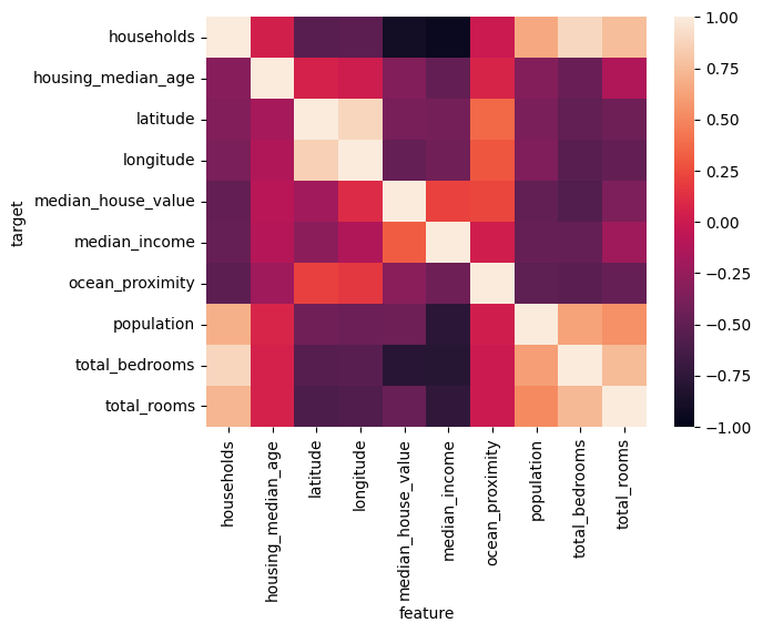
import seaborn as sns
sns.heatmap(beyond_corr, vmin=-1, vmax=1)
<Axes: xlabel='feature', ylabel='target'>