Machine learning fairness

Machine Learning fairness is an important part of modern day data modeling. Here we explore an introduction to make models more fair and equitable.

Machine learning is a powerful tool that has revolutionized many industries by enabling computers to learn from data and make predictions or decisions.

However, as machine learning algorithms become increasingly ubiquitous in our daily lives, concerns about fairness and equity have emerged. Machine learning fairness refers to the idea that machine learning models should not perpetuate or exacerbate existing biases or discrimination. Fairness means that the model treats all individuals or groups fairly, regardless of race, gender, ethnicity, or other protected characteristics.

This notebook will provide an overview of the key concepts and challenges in machine learning fairness, as well as some techniques commonly used to address them.

How To

from sklearn.model_selection import train_test_split
import pandas as pd

df = pd.read_csv("data/housing.csv").dropna()
df.head()

	longitude	latitude	housing_median_age	total_rooms	total_bedrooms	population	households	median_income	median_house_value	ocean_proximity
0	-122.23	37.88	41.0	880.0	129.0	322.0	126.0	8.3252	452600.0	NEAR BAY
1	-122.22	37.86	21.0	7099.0	1106.0	2401.0	1138.0	8.3014	358500.0	NEAR BAY
2	-122.24	37.85	52.0	1467.0	190.0	496.0	177.0	7.2574	352100.0	NEAR BAY
3	-122.25	37.85	52.0	1274.0	235.0	558.0	219.0	5.6431	341300.0	NEAR BAY
4	-122.25	37.85	52.0	1627.0	280.0	565.0	259.0	3.8462	342200.0	NEAR BAY

x_train, x_, y_train, y_ = train_test_split(df.drop(["longitude","latitude", "ocean_proximity", "median_house_value"], axis=1), 
                                                    df.median_house_value, test_size=.5, stratify=df.ocean_proximity)

x_val, x_test, y_val, y_test = train_test_split(x_, y_, test_size=.5)

from sklearn.ensemble import RandomForestRegressor
model = RandomForestRegressor().fit(x_train, y_train)

model.score(x_val, y_val)

0.6586735958677061

from sklearn.model_selection import cross_val_score

for cls in df.ocean_proximity.unique():
    print(cls)
    try:
        idx = df[df.ocean_proximity.isin([cls])].index

        idx_val = x_val.index.intersection(idx)
        print(model.score(x_val.loc[idx_val, :], y_val.loc[idx_val]))

        val = cross_val_score(model, x_val.loc[idx_val, :], y_val.loc[idx_val])
        print(val)
        print(val.mean(), " +- ", val.std(), "\n")
    except:
        print("Error in Validation")
    try:
        idx = df[df.ocean_proximity.isin([cls])].index

        idx_test = x_test.index.intersection(idx)
        print(model.score(x_test.loc[idx_test, :], y_test.loc[idx_test]))
        
        tst = cross_val_score(model,x_test.loc[idx_test, :], y_test.loc[idx_test])
        print(tst)
        print(tst.mean(), " +- ", tst.std(), "\n")
    except:
        print("Error in Test")

NEAR BAY
0.6914888806800314

[0.51361569 0.64630664 0.59280962 0.69167432 0.66258008]
0.621397271310316  +-  0.06275266873707354 

0.5750599987255491

[0.46930571 0.43675151 0.56149112 0.53991517 0.43855913]
0.4892045308559778  +-  0.05197914753138655 

<1H OCEAN
0.6164340776775521

[0.62935218 0.58064886 0.57057219 0.62693846 0.66328712]
0.6141597616245293  +-  0.034148086465257306 

0.6191524643956172

[0.62363128 0.61138027 0.60811331 0.57578551 0.60926118]
0.6056343121336554  +-  0.015919533470271377 

INLAND
0.1967543190323986

[0.60097059 0.43543378 0.47527694 0.48630933 0.57854818]
0.5153077647383298  +-  0.06349913017713156 

0.20640897263306657

[0.47371532 0.54227822 0.23409711 0.52081891 0.43949161]
0.4420802336257415  +-  0.1100035220041293 

NEAR OCEAN
0.5441817718762696

[0.56994925 0.62178888 0.52010515 0.50148382 0.57472886]
0.5576111924627768  +-  0.042710663438220095 

0.6036955726079807

[0.5883007  0.61904115 0.55511549 0.49335263 0.55245425]
0.5616528456131616  +-  0.04194233268167542 

ISLAND
-4.747812762984071
Error in Validation
nan
Error in Test

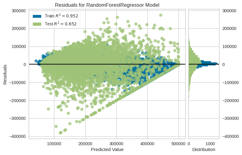
Calculate Residuals

from yellowbrick.regressor import residuals_plot, prediction_error

residuals_plot(model, x_train, y_train, x_test, y_test)

---------------------------------------------------------------------------
AttributeError                            Traceback (most recent call last)
File /opt/hostedtoolcache/Python/3.8.18/x64/lib/python3.8/site-packages/yellowbrick/utils/wrapper.py:48, in Wrapper.__getattr__(self, attr)
     47 try:
---> 48     return getattr(self._wrapped, attr)
     49 except AttributeError as e:

AttributeError: 'RandomForestRegressor' object has no attribute 'line_color'

The above exception was the direct cause of the following exception:

YellowbrickAttributeError                 Traceback (most recent call last)
File /opt/hostedtoolcache/Python/3.8.18/x64/lib/python3.8/site-packages/IPython/core/formatters.py:974, in MimeBundleFormatter.__call__(self, obj, include, exclude)
    971     method = get_real_method(obj, self.print_method)
    973     if method is not None:
--> 974         return method(include=include, exclude=exclude)
    975     return None
    976 else:

File /opt/hostedtoolcache/Python/3.8.18/x64/lib/python3.8/site-packages/sklearn/base.py:669, in BaseEstimator._repr_mimebundle_(self, **kwargs)
    667 def _repr_mimebundle_(self, **kwargs):
    668     """Mime bundle used by jupyter kernels to display estimator"""
--> 669     output = {"text/plain": repr(self)}
    670     if get_config()["display"] == "diagram":
    671         output["text/html"] = estimator_html_repr(self)

File /opt/hostedtoolcache/Python/3.8.18/x64/lib/python3.8/site-packages/sklearn/base.py:287, in BaseEstimator.__repr__(self, N_CHAR_MAX)
    279 # use ellipsis for sequences with a lot of elements
    280 pp = _EstimatorPrettyPrinter(
    281     compact=True,
    282     indent=1,
    283     indent_at_name=True,
    284     n_max_elements_to_show=N_MAX_ELEMENTS_TO_SHOW,
    285 )
--> 287 repr_ = pp.pformat(self)
    289 # Use bruteforce ellipsis when there are a lot of non-blank characters
    290 n_nonblank = len("".join(repr_.split()))

File /opt/hostedtoolcache/Python/3.8.18/x64/lib/python3.8/pprint.py:153, in PrettyPrinter.pformat(self, object)
    151 def pformat(self, object):
    152     sio = _StringIO()
--> 153     self._format(object, sio, 0, 0, {}, 0)
    154     return sio.getvalue()

File /opt/hostedtoolcache/Python/3.8.18/x64/lib/python3.8/pprint.py:170, in PrettyPrinter._format(self, object, stream, indent, allowance, context, level)
    168     self._readable = False
    169     return
--> 170 rep = self._repr(object, context, level)
    171 max_width = self._width - indent - allowance
    172 if len(rep) > max_width:

File /opt/hostedtoolcache/Python/3.8.18/x64/lib/python3.8/pprint.py:404, in PrettyPrinter._repr(self, object, context, level)
    403 def _repr(self, object, context, level):
--> 404     repr, readable, recursive = self.format(object, context.copy(),
    405                                             self._depth, level)
    406     if not readable:
    407         self._readable = False

File /opt/hostedtoolcache/Python/3.8.18/x64/lib/python3.8/site-packages/sklearn/utils/_pprint.py:189, in _EstimatorPrettyPrinter.format(self, object, context, maxlevels, level)
    188 def format(self, object, context, maxlevels, level):
--> 189     return _safe_repr(
    190         object, context, maxlevels, level, changed_only=self._changed_only
    191     )

File /opt/hostedtoolcache/Python/3.8.18/x64/lib/python3.8/site-packages/sklearn/utils/_pprint.py:440, in _safe_repr(object, context, maxlevels, level, changed_only)
    438 recursive = False
    439 if changed_only:
--> 440     params = _changed_params(object)
    441 else:
    442     params = object.get_params(deep=False)

File /opt/hostedtoolcache/Python/3.8.18/x64/lib/python3.8/site-packages/sklearn/utils/_pprint.py:93, in _changed_params(estimator)
     89 def _changed_params(estimator):
     90     """Return dict (param_name: value) of parameters that were given to
     91     estimator with non-default values."""
---> 93     params = estimator.get_params(deep=False)
     94     init_func = getattr(estimator.__init__, "deprecated_original", estimator.__init__)
     95     init_params = inspect.signature(init_func).parameters

File /opt/hostedtoolcache/Python/3.8.18/x64/lib/python3.8/site-packages/yellowbrick/base.py:342, in ModelVisualizer.get_params(self, deep)
    334 def get_params(self, deep=True):
    335     """
    336     After v0.24 - scikit-learn is able to determine that ``self.estimator`` is
    337     nested and fetches its params using ``estimator__param``. This functionality is
   (...)
    340     the estimator params.
    341     """
--> 342     params = super(ModelVisualizer, self).get_params(deep=deep)
    343     for param in list(params.keys()):
    344         if param.startswith("estimator__"):

File /opt/hostedtoolcache/Python/3.8.18/x64/lib/python3.8/site-packages/sklearn/base.py:195, in BaseEstimator.get_params(self, deep)
    193 out = dict()
    194 for key in self._get_param_names():
--> 195     value = getattr(self, key)
    196     if deep and hasattr(value, "get_params") and not isinstance(value, type):
    197         deep_items = value.get_params().items()

File /opt/hostedtoolcache/Python/3.8.18/x64/lib/python3.8/site-packages/yellowbrick/utils/wrapper.py:50, in Wrapper.__getattr__(self, attr)
     48     return getattr(self._wrapped, attr)
     49 except AttributeError as e:
---> 50     raise YellowbrickAttributeError(f"neither visualizer '{self.__class__.__name__}' nor wrapped estimator '{type(self._wrapped).__name__}' have attribute '{attr}'") from e

YellowbrickAttributeError: neither visualizer 'ResidualsPlot' nor wrapped estimator 'RandomForestRegressor' have attribute 'line_color'

---------------------------------------------------------------------------
AttributeError                            Traceback (most recent call last)
File /opt/hostedtoolcache/Python/3.8.18/x64/lib/python3.8/site-packages/yellowbrick/utils/wrapper.py:48, in Wrapper.__getattr__(self, attr)
     47 try:
---> 48     return getattr(self._wrapped, attr)
     49 except AttributeError as e:

AttributeError: 'RandomForestRegressor' object has no attribute 'line_color'

The above exception was the direct cause of the following exception:

YellowbrickAttributeError                 Traceback (most recent call last)
File /opt/hostedtoolcache/Python/3.8.18/x64/lib/python3.8/site-packages/IPython/core/formatters.py:708, in PlainTextFormatter.__call__(self, obj)
    701 stream = StringIO()
    702 printer = pretty.RepresentationPrinter(stream, self.verbose,
    703     self.max_width, self.newline,
    704     max_seq_length=self.max_seq_length,
    705     singleton_pprinters=self.singleton_printers,
    706     type_pprinters=self.type_printers,
    707     deferred_pprinters=self.deferred_printers)
--> 708 printer.pretty(obj)
    709 printer.flush()
    710 return stream.getvalue()

File /opt/hostedtoolcache/Python/3.8.18/x64/lib/python3.8/site-packages/IPython/lib/pretty.py:410, in RepresentationPrinter.pretty(self, obj)
    407                         return meth(obj, self, cycle)
    408                 if cls is not object \
    409                         and callable(cls.__dict__.get('__repr__')):
--> 410                     return _repr_pprint(obj, self, cycle)
    412     return _default_pprint(obj, self, cycle)
    413 finally:

File /opt/hostedtoolcache/Python/3.8.18/x64/lib/python3.8/site-packages/IPython/lib/pretty.py:778, in _repr_pprint(obj, p, cycle)
    776 """A pprint that just redirects to the normal repr function."""
    777 # Find newlines and replace them with p.break_()
--> 778 output = repr(obj)
    779 lines = output.splitlines()
    780 with p.group():

File /opt/hostedtoolcache/Python/3.8.18/x64/lib/python3.8/site-packages/sklearn/base.py:287, in BaseEstimator.__repr__(self, N_CHAR_MAX)
    279 # use ellipsis for sequences with a lot of elements
    280 pp = _EstimatorPrettyPrinter(
    281     compact=True,
    282     indent=1,
    283     indent_at_name=True,
    284     n_max_elements_to_show=N_MAX_ELEMENTS_TO_SHOW,
    285 )
--> 287 repr_ = pp.pformat(self)
    289 # Use bruteforce ellipsis when there are a lot of non-blank characters
    290 n_nonblank = len("".join(repr_.split()))

File /opt/hostedtoolcache/Python/3.8.18/x64/lib/python3.8/pprint.py:153, in PrettyPrinter.pformat(self, object)
    151 def pformat(self, object):
    152     sio = _StringIO()
--> 153     self._format(object, sio, 0, 0, {}, 0)
    154     return sio.getvalue()

File /opt/hostedtoolcache/Python/3.8.18/x64/lib/python3.8/pprint.py:170, in PrettyPrinter._format(self, object, stream, indent, allowance, context, level)
    168     self._readable = False
    169     return
--> 170 rep = self._repr(object, context, level)
    171 max_width = self._width - indent - allowance
    172 if len(rep) > max_width:

File /opt/hostedtoolcache/Python/3.8.18/x64/lib/python3.8/pprint.py:404, in PrettyPrinter._repr(self, object, context, level)
    403 def _repr(self, object, context, level):
--> 404     repr, readable, recursive = self.format(object, context.copy(),
    405                                             self._depth, level)
    406     if not readable:
    407         self._readable = False

File /opt/hostedtoolcache/Python/3.8.18/x64/lib/python3.8/site-packages/sklearn/utils/_pprint.py:189, in _EstimatorPrettyPrinter.format(self, object, context, maxlevels, level)
    188 def format(self, object, context, maxlevels, level):
--> 189     return _safe_repr(
    190         object, context, maxlevels, level, changed_only=self._changed_only
    191     )

File /opt/hostedtoolcache/Python/3.8.18/x64/lib/python3.8/site-packages/sklearn/utils/_pprint.py:440, in _safe_repr(object, context, maxlevels, level, changed_only)
    438 recursive = False
    439 if changed_only:
--> 440     params = _changed_params(object)
    441 else:
    442     params = object.get_params(deep=False)

File /opt/hostedtoolcache/Python/3.8.18/x64/lib/python3.8/site-packages/sklearn/utils/_pprint.py:93, in _changed_params(estimator)
     89 def _changed_params(estimator):
     90     """Return dict (param_name: value) of parameters that were given to
     91     estimator with non-default values."""
---> 93     params = estimator.get_params(deep=False)
     94     init_func = getattr(estimator.__init__, "deprecated_original", estimator.__init__)
     95     init_params = inspect.signature(init_func).parameters

File /opt/hostedtoolcache/Python/3.8.18/x64/lib/python3.8/site-packages/yellowbrick/base.py:342, in ModelVisualizer.get_params(self, deep)
    334 def get_params(self, deep=True):
    335     """
    336     After v0.24 - scikit-learn is able to determine that ``self.estimator`` is
    337     nested and fetches its params using ``estimator__param``. This functionality is
   (...)
    340     the estimator params.
    341     """
--> 342     params = super(ModelVisualizer, self).get_params(deep=deep)
    343     for param in list(params.keys()):
    344         if param.startswith("estimator__"):

File /opt/hostedtoolcache/Python/3.8.18/x64/lib/python3.8/site-packages/sklearn/base.py:195, in BaseEstimator.get_params(self, deep)
    193 out = dict()
    194 for key in self._get_param_names():
--> 195     value = getattr(self, key)
    196     if deep and hasattr(value, "get_params") and not isinstance(value, type):
    197         deep_items = value.get_params().items()

File /opt/hostedtoolcache/Python/3.8.18/x64/lib/python3.8/site-packages/yellowbrick/utils/wrapper.py:50, in Wrapper.__getattr__(self, attr)
     48     return getattr(self._wrapped, attr)
     49 except AttributeError as e:
---> 50     raise YellowbrickAttributeError(f"neither visualizer '{self.__class__.__name__}' nor wrapped estimator '{type(self._wrapped).__name__}' have attribute '{attr}'") from e

YellowbrickAttributeError: neither visualizer 'ResidualsPlot' nor wrapped estimator 'RandomForestRegressor' have attribute 'line_color'

---------------------------------------------------------------------------
AttributeError                            Traceback (most recent call last)
File /opt/hostedtoolcache/Python/3.8.18/x64/lib/python3.8/site-packages/yellowbrick/utils/wrapper.py:48, in Wrapper.__getattr__(self, attr)
     47 try:
---> 48     return getattr(self._wrapped, attr)
     49 except AttributeError as e:

AttributeError: 'RandomForestRegressor' object has no attribute 'line_color'

The above exception was the direct cause of the following exception:

YellowbrickAttributeError                 Traceback (most recent call last)
File /opt/hostedtoolcache/Python/3.8.18/x64/lib/python3.8/site-packages/IPython/core/formatters.py:344, in BaseFormatter.__call__(self, obj)
    342     method = get_real_method(obj, self.print_method)
    343     if method is not None:
--> 344         return method()
    345     return None
    346 else:

File /opt/hostedtoolcache/Python/3.8.18/x64/lib/python3.8/site-packages/sklearn/base.py:665, in BaseEstimator._repr_html_inner(self)
    660 def _repr_html_inner(self):
    661     """This function is returned by the @property `_repr_html_` to make
    662     `hasattr(estimator, "_repr_html_") return `True` or `False` depending
    663     on `get_config()["display"]`.
    664     """
--> 665     return estimator_html_repr(self)

File /opt/hostedtoolcache/Python/3.8.18/x64/lib/python3.8/site-packages/sklearn/utils/_estimator_html_repr.py:388, in estimator_html_repr(estimator)
    386 style_template = Template(_STYLE)
    387 style_with_id = style_template.substitute(id=container_id)
--> 388 estimator_str = str(estimator)
    390 # The fallback message is shown by default and loading the CSS sets
    391 # div.sk-text-repr-fallback to display: none to hide the fallback message.
    392 #
   (...)
    397 # The reverse logic applies to HTML repr div.sk-container.
    398 # div.sk-container is hidden by default and the loading the CSS displays it.
    399 fallback_msg = (
    400     "In a Jupyter environment, please rerun this cell to show the HTML"
    401     " representation or trust the notebook. <br />On GitHub, the"
    402     " HTML representation is unable to render, please try loading this page"
    403     " with nbviewer.org."
    404 )

File /opt/hostedtoolcache/Python/3.8.18/x64/lib/python3.8/site-packages/sklearn/base.py:287, in BaseEstimator.__repr__(self, N_CHAR_MAX)
    279 # use ellipsis for sequences with a lot of elements
    280 pp = _EstimatorPrettyPrinter(
    281     compact=True,
    282     indent=1,
    283     indent_at_name=True,
    284     n_max_elements_to_show=N_MAX_ELEMENTS_TO_SHOW,
    285 )
--> 287 repr_ = pp.pformat(self)
    289 # Use bruteforce ellipsis when there are a lot of non-blank characters
    290 n_nonblank = len("".join(repr_.split()))

File /opt/hostedtoolcache/Python/3.8.18/x64/lib/python3.8/pprint.py:153, in PrettyPrinter.pformat(self, object)
    151 def pformat(self, object):
    152     sio = _StringIO()
--> 153     self._format(object, sio, 0, 0, {}, 0)
    154     return sio.getvalue()

File /opt/hostedtoolcache/Python/3.8.18/x64/lib/python3.8/pprint.py:170, in PrettyPrinter._format(self, object, stream, indent, allowance, context, level)
    168     self._readable = False
    169     return
--> 170 rep = self._repr(object, context, level)
    171 max_width = self._width - indent - allowance
    172 if len(rep) > max_width:

File /opt/hostedtoolcache/Python/3.8.18/x64/lib/python3.8/pprint.py:404, in PrettyPrinter._repr(self, object, context, level)
    403 def _repr(self, object, context, level):
--> 404     repr, readable, recursive = self.format(object, context.copy(),
    405                                             self._depth, level)
    406     if not readable:
    407         self._readable = False

File /opt/hostedtoolcache/Python/3.8.18/x64/lib/python3.8/site-packages/sklearn/utils/_pprint.py:189, in _EstimatorPrettyPrinter.format(self, object, context, maxlevels, level)
    188 def format(self, object, context, maxlevels, level):
--> 189     return _safe_repr(
    190         object, context, maxlevels, level, changed_only=self._changed_only
    191     )

File /opt/hostedtoolcache/Python/3.8.18/x64/lib/python3.8/site-packages/sklearn/utils/_pprint.py:440, in _safe_repr(object, context, maxlevels, level, changed_only)
    438 recursive = False
    439 if changed_only:
--> 440     params = _changed_params(object)
    441 else:
    442     params = object.get_params(deep=False)

File /opt/hostedtoolcache/Python/3.8.18/x64/lib/python3.8/site-packages/sklearn/utils/_pprint.py:93, in _changed_params(estimator)
     89 def _changed_params(estimator):
     90     """Return dict (param_name: value) of parameters that were given to
     91     estimator with non-default values."""
---> 93     params = estimator.get_params(deep=False)
     94     init_func = getattr(estimator.__init__, "deprecated_original", estimator.__init__)
     95     init_params = inspect.signature(init_func).parameters

File /opt/hostedtoolcache/Python/3.8.18/x64/lib/python3.8/site-packages/yellowbrick/base.py:342, in ModelVisualizer.get_params(self, deep)
    334 def get_params(self, deep=True):
    335     """
    336     After v0.24 - scikit-learn is able to determine that ``self.estimator`` is
    337     nested and fetches its params using ``estimator__param``. This functionality is
   (...)
    340     the estimator params.
    341     """
--> 342     params = super(ModelVisualizer, self).get_params(deep=deep)
    343     for param in list(params.keys()):
    344         if param.startswith("estimator__"):

File /opt/hostedtoolcache/Python/3.8.18/x64/lib/python3.8/site-packages/sklearn/base.py:195, in BaseEstimator.get_params(self, deep)
    193 out = dict()
    194 for key in self._get_param_names():
--> 195     value = getattr(self, key)
    196     if deep and hasattr(value, "get_params") and not isinstance(value, type):
    197         deep_items = value.get_params().items()

File /opt/hostedtoolcache/Python/3.8.18/x64/lib/python3.8/site-packages/yellowbrick/utils/wrapper.py:50, in Wrapper.__getattr__(self, attr)
     48     return getattr(self._wrapped, attr)
     49 except AttributeError as e:
---> 50     raise YellowbrickAttributeError(f"neither visualizer '{self.__class__.__name__}' nor wrapped estimator '{type(self._wrapped).__name__}' have attribute '{attr}'") from e

YellowbrickAttributeError: neither visualizer 'ResidualsPlot' nor wrapped estimator 'RandomForestRegressor' have attribute 'line_color'

prediction_error(model, x_train, y_train, x_test, y_test)

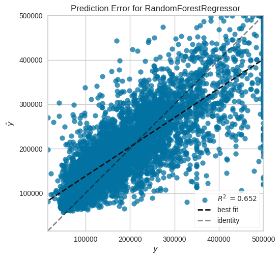
PredictionError(ax=<Axes: title={'center': 'Prediction Error for RandomForestRegressor'}, xlabel='$y$', ylabel='$\\hat{y}$'>,
                estimator=RandomForestRegressor())

In a Jupyter environment, please rerun this cell to show the HTML representation or trust the notebook.
On GitHub, the HTML representation is unable to render, please try loading this page with nbviewer.org.

Confusion Matrix for Classifiers

from sklearn.metrics import plot_confusion_matrix

---------------------------------------------------------------------------
ImportError                               Traceback (most recent call last)
Cell In[10], line 1
----> 1 from sklearn.metrics import plot_confusion_matrix

ImportError: cannot import name 'plot_confusion_matrix' from 'sklearn.metrics' (/opt/hostedtoolcache/Python/3.8.18/x64/lib/python3.8/site-packages/sklearn/metrics/__init__.py)

from sklearn.ensemble import RandomForestClassifier

x_train, x_, y_train, y_ = train_test_split(df.drop(["longitude","latitude", "ocean_proximity"], axis=1), 
                                                    df.ocean_proximity, test_size=.5, stratify=df.ocean_proximity)

x_val, x_test, y_val, y_test = train_test_split(x_, y_, test_size=.5)

model = RandomForestClassifier().fit(x_train, y_train)

plot_confusion_matrix(model, x_test, y_test)

---------------------------------------------------------------------------
NameError                                 Traceback (most recent call last)
Cell In[12], line 1
----> 1 plot_confusion_matrix(model, x_test, y_test)

NameError: name 'plot_confusion_matrix' is not defined

plot_confusion_matrix(model, x_test, y_test, normalize="all")

---------------------------------------------------------------------------
NameError                                 Traceback (most recent call last)
Cell In[13], line 1
----> 1 plot_confusion_matrix(model, x_test, y_test, normalize="all")

NameError: name 'plot_confusion_matrix' is not defined

Other Visualizations that are important

from yellowbrick.classifier import confusion_matrix, classification_report, precision_recall_curve, roc_auc

confusion_matrix(model, x_train, y_train, x_test, y_test)

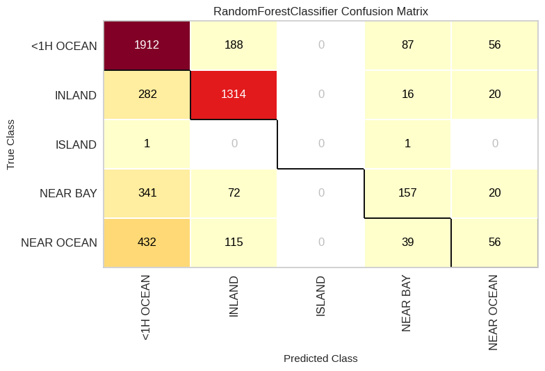
ConfusionMatrix(ax=<Axes: title={'center': 'RandomForestClassifier Confusion Matrix'}, xlabel='Predicted Class', ylabel='True Class'>,
                cmap=<matplotlib.colors.ListedColormap object at 0x7fa324633b50>,
                estimator=RandomForestClassifier())

In a Jupyter environment, please rerun this cell to show the HTML representation or trust the notebook.
On GitHub, the HTML representation is unable to render, please try loading this page with nbviewer.org.

classification_report(model, x_train, y_train, x_test, y_test)

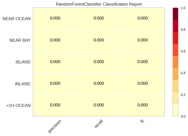
ClassificationReport(ax=<Axes: title={'center': 'RandomForestClassifier Classification Report'}>,
                     cmap=<matplotlib.colors.ListedColormap object at 0x7fa324481190>,
                     estimator=RandomForestClassifier())

In a Jupyter environment, please rerun this cell to show the HTML representation or trust the notebook.
On GitHub, the HTML representation is unable to render, please try loading this page with nbviewer.org.

from sklearn.metrics import classification_report

print(classification_report(y_test, model.predict(x_test)))

              precision    recall  f1-score   support

   <1H OCEAN       0.64      0.85      0.73      2243
      INLAND       0.78      0.81      0.79      1632
      ISLAND       0.00      0.00      0.00         2
    NEAR BAY       0.52      0.27      0.35       590
  NEAR OCEAN       0.37      0.09      0.14       642

    accuracy                           0.67      5109
   macro avg       0.46      0.40      0.40      5109
weighted avg       0.64      0.67      0.63      5109

precision_recall_curve(model, x_train, y_train, x_test, y_test)

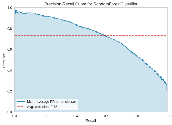
PrecisionRecallCurve(ax=<Axes: title={'center': 'Precision-Recall Curve for RandomForestClassifier'}, xlabel='Recall', ylabel='Precision'>,
                     estimator=OneVsRestClassifier(estimator=RandomForestClassifier()),
                     iso_f1_values={0.2, 0.4, 0.6, 0.8})

In a Jupyter environment, please rerun this cell to show the HTML representation or trust the notebook.
On GitHub, the HTML representation is unable to render, please try loading this page with nbviewer.org.

roc_auc(model, x_train, y_train, x_test, y_test)

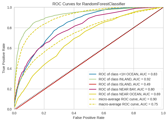
ROCAUC(ax=<Axes: title={'center': 'ROC Curves for RandomForestClassifier'}, xlabel='False Positive Rate', ylabel='True Positive Rate'>,
       estimator=RandomForestClassifier())

In a Jupyter environment, please rerun this cell to show the HTML representation or trust the notebook.
On GitHub, the HTML representation is unable to render, please try loading this page with nbviewer.org.

Exercise

Modify the code to generate dummy models for each class.

Additional Resources

• ML Fairness

• ML Fairness Gym

• F A T M L